Category: Library

Foundations · 02

What you will build

The twisting tower is the “hello world” of Grasshopper for good reason: in sixteen components it demonstrates the whole logic of parametric modelling — one piece of source geometry, a stream of numbers, a chain of transformations, a skin. Change any slider and the tower rebuilds itself instantly.

You will stack a rectangular floor plate into thirty storeys, rotate each storey a little more than the one below, loft the result into a twisting envelope, and bake it into Rhino as real geometry. More importantly, you will understand what every wire carries. The build is identical in Rhino 7 and Rhino 8 — nothing here is version-specific.

Reading the canvas before you start

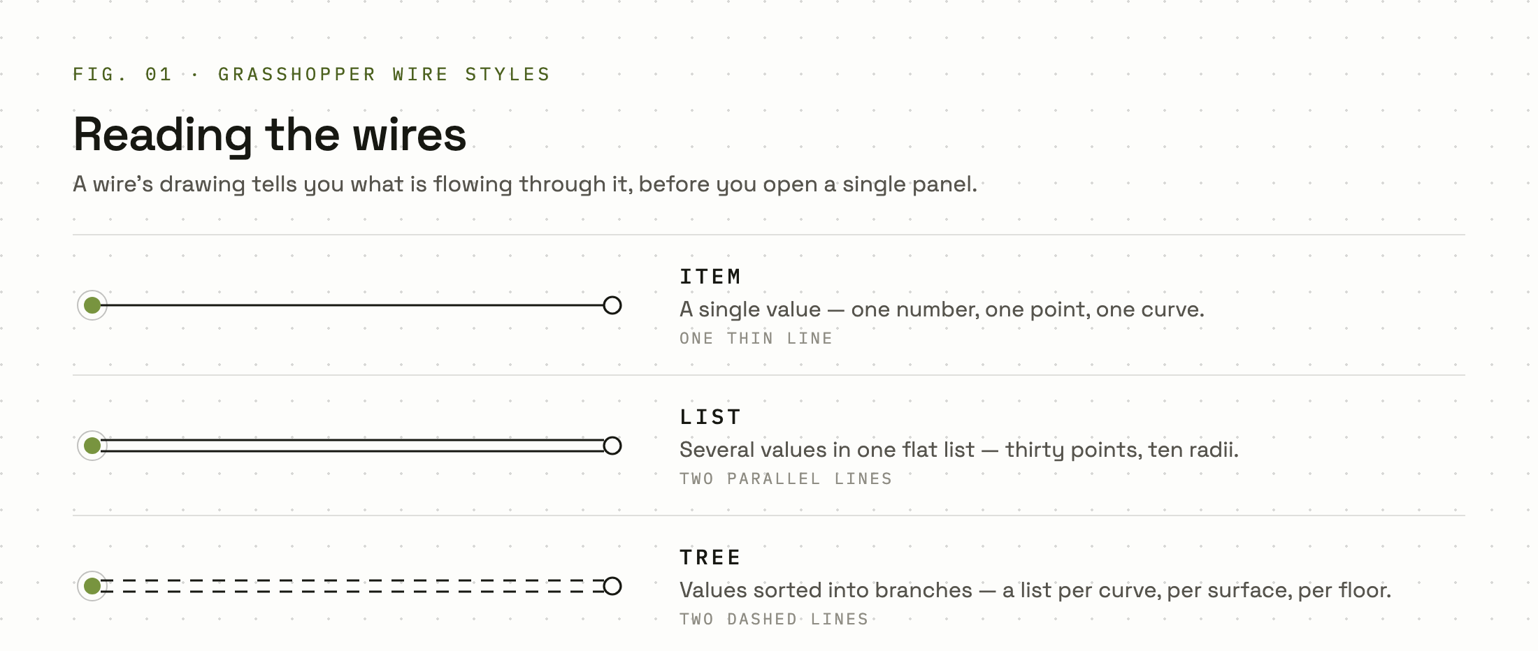
A quick orientation, because we will talk about wires constantly. Every component has inputs on its left edge and outputs on its right; a wire always flows from an output to an input. With fancy wires on (Display menu, Draw Fancy Wires — enabled by default), the wire tells you what it carries: a single line means one item, a double line means a list, and a dashed double line means a data tree (we meet those in a later tutorial). Watching a wire change from single to double is the fastest way to see what your definition is really doing.

To place a component, double-click an empty patch of canvas and type its name, or find it on the tabbed toolbar. I give the name and tab location for everything we use.

Step 1: A centred footprint

The tower starts as a single rectangle. The Rectangle component (Curve tab, Primitive panel) draws one on a base plane — by default the World XY plane at the origin. One subtlety matters: its X Size and Y Size inputs accept a domain, a numeric interval. Feed a plain number such as 12 and Grasshopper reads it as the domain 0 to 12, putting a corner at the origin. Since we will twist the tower about the vertical axis through the origin, we want the rectangle centred there — otherwise every floor swings around its own corner.

1. Double-click the canvas, type 2.0<6.0<15.0 and press Enter. This shortcut creates a Number Slider with minimum 2, value 6, maximum 15; the decimal points make it a floating-point slider. Rename it (double-click its label) to Half width.
2. Place a Negative component (Maths tab, Operators panel) and wire the slider into its input. It flips the sign: 6 becomes −6.
3. Place a Construct Domain component (Maths tab, Domain panel). Wire Negative’s output into A and the slider directly into B. Output I is now the interval −6 to 6.
4. Place a Rectangle and wire Construct Domain’s I into both the X and Y inputs. One output can feed any number of inputs — your first taste of wire reuse.

Slider "Half width" (6.0) → Negative (x)
Negative (y) → Construct Domain (A)
Slider "Half width" (6.0) → Construct Domain (B)
Construct Domain (I) → Rectangle (X)
Construct Domain (I) → Rectangle (Y)

You should see a 12 × 12 square centred on the origin. Every wire so far carries a single item, so every wire draws as a single line. Drag the slider and the square resizes symmetrically — exactly what the Construct Domain detour bought us.

Step 2: One counter drives everything

A tower is repetition, and repetition in Grasshopper means a list of numbers. The Series component (Sets tab, Sequence panel) generates an arithmetic sequence from S (start), N (step) and C (count). Rather than one series of elevations and another of angles, we generate a single series of floor indices — 0, 1, 2, 3 … — and multiply it by different factors downstream. One counting stream, many uses.

1. Type 1<30<60 on the canvas — whole numbers ask for an integer slider, which is what a floor count should be. Rename it Floors.
2. Place a Series component. Leave S at 0 and N at 1, and wire Floors into C.
3. Place a Panel (Params tab, Input panel) and wire the Series output S into it. You should read 0, 1, 2 … 29.

Look at the wire leaving Series: it is now a double line, because it carries thirty numbers. Hanging a Panel off any output you are unsure about is the single most useful debugging move in Grasshopper.

Step 3: Stacking the floors with Move

To stack the rectangle we need vertical vectors, one per floor, each longer than the last. Unit Z (Vector tab, Vector panel) produces a vector pointing straight up, and its F (factor) input scales its length. Feed it one number and you get one vector; feed it thirty numbers and you get thirty vectors. Components handle lists automatically — no loops to write.

1. Create a slider by typing 2.5<3.5<5.0; rename it Floor height.
2. Place a Multiplication component (Maths tab, Operators panel). Wire the Series output S into A and Floor height into B. The result is a list of elevations: 0, 3.5, 7, 10.5 …
3. Place Unit Z and wire the Multiplication result R into F.
4. Place a Move component (Transform tab, Euclidean panel). Wire the Rectangle output R into G (geometry) and Unit Z’s V into T (motion).

Series (S) → Multiplication (A)
Slider "Floor height" (3.5) → Multiplication (B)
Multiplication (R) → Unit Z (F)
Unit Z (V) → Move (T)
Rectangle (R) → Move (G)

Pause on what happened inside Move, because it is the heart of how Grasshopper thinks. Its G input received one rectangle; its T input received thirty vectors. When list lengths disagree, Grasshopper repeats the last item of the shorter list, so the single rectangle is reused for every vector and Move outputs thirty copies at thirty elevations. You never asked for copies — the data matching produced them. The viewport now shows a clean stack of squares, and the wire leaving Move’s G output is a double line.

Step 4: The twist

Now the signature move. Rotate (Transform tab, Euclidean panel) spins geometry in the plane fed into its P input — and its default, World XY, has its axis running straight up the centre of our stack. All we need is a list of graduated angles: floor 0 rotates 0°, floor 1 rotates 3°, floor 2 rotates 6°, and so on. Our index series multiplied by a twist increment gives exactly that.

One trap: Rotate expects its angle in radians. The clearest fix is the Radians component (Maths tab, Trig panel), which converts degrees to radians in plain sight. (You can also right-click an angle input and tick Degrees, but hidden switches make definitions harder for colleagues to read — prefer the explicit component while learning.)

1. Create a slider by typing 0.0<3.0<12.0; rename it Twist per floor. This is degrees of rotation added per storey.
2. Place a second Multiplication. Wire the same Series output S into A — the counting stream now does double duty — and Twist per floor into B.
3. Place a Radians component and wire the Multiplication result R into its D input.
4. Place Rotate. Wire Move’s G into Rotate’s G, and Radians’ R into Rotate’s A. Leave P untouched.

Series (S) → Multiplication #2 (A)
Slider "Twist per floor" (3.0) → Multiplication #2 (B)
Multiplication #2 (R) → Radians (D)
Radians (R) → Rotate (A)
Move (G) → Rotate (G)

This time the matching is one-to-one: thirty rectangles meet thirty angles, so each floor gets its own rotation, and the stack spirals. We moved first and rotated second, but here the order would not matter — a vertical translation and a rotation about the vertical axis are independent. That is a special case: in general, transformation order matters a great deal.

Step 5: Skinning with Loft

The Loft component (Surface tab, Freeform panel) stretches a surface through an ordered list of section curves — exactly what Rotate is handing us. Wire Rotate’s G into Loft’s C (curves) input and leave O (options) at its defaults. Because every section is a copy of the same closed rectangle, seams and curve directions already line up, and the loft closes into a clean twisted tube.

Rotate (G) → Loft (C)

The viewport looks busy because Grasshopper previews every component at once. Right-click Move and Rotate and untick Preview to hide the intermediate rectangles. Now play: wind and unwind Twist per floor, push Floors to 60, squeeze Half width down. Every change ripples through the whole wire chain in real time. You have not modelled a tower — you have modelled the rules for a family of towers.

Baking the result

Everything so far is preview only. It lives inside the definition; Rhino cannot select it, snap to it, render or export it, and if you close the definition it vanishes. To turn preview into real Rhino geometry, you bake it.

1. Right-click the Loft component and choose Bake…
2. In the dialogue, choose a target layer — a dedicated layer such as GH Bake keeps baked output from tangling with your working model.
3. Click OK. The twisted envelope is now an ordinary polysurface in the Rhino document.

Two things to understand about baking. First, it is a one-way copy: the baked object is frozen, and moving a slider afterwards changes the preview but not the baked geometry. If you refine the design, bake again — and delete the stale version, or you will accumulate overlapping towers. Second, you can bake from any component. Right-click Rotate and bake it, and you get thirty floor-plate outlines as curves, ready for drawings.

---

Practice

• Taper the tower. Multiply the Series output by a small negative number and add it to Half width with an Addition component (Maths tab, Operators panel). Feed that per-floor width into Negative and Construct Domain in place of the slider: Rectangle now receives thirty domains, so thirty different-sized rectangles exist before Move even sees them.
• Break it on purpose. Wire the elevations (the first Multiplication’s output) into Rotate’s A instead of the Radians output, and explain to yourself exactly why the tower knots up. Reading a broken definition is a skill you will use weekly.
• Rebuild from memory. Open a blank canvas and reconstruct the definition without looking. If you can narrate what each wire carries — one rectangle, thirty numbers, thirty vectors, thirty angles — the lesson has stuck.

Next in the Foundations track we open up the thing this tutorial quietly relied on: how Grasshopper matches lists of different lengths, and how to take control of it. Members can find the completed definition, the tapered variant, and all course files in the Members Library.

Foundations · 01

Grasshopper is not a modelling tool. It is a tool for describing how a model should be built, so the model can rebuild itself every time you change your mind. Instead of drawing a circle, you place a component that makes circles, feed it a radius, and let Rhino draw the result. Change the radius and the circle updates instantly — along with everything downstream of it. That single idea, geometry as the output of a live definition rather than a frozen drawing, is what makes parametric design worth learning.

Before any of that pays off, you need to be comfortable in the interface. This first tutorial is a guided walk around the Grasshopper environment: the canvas, the component ribbon, parameters versus components, wires, and the shortcuts fluent users lean on. By the end you will have built a small working definition and know where everything lives.

Opening Grasshopper

Grasshopper ships inside Rhino — there is nothing extra to install. Start Rhino, type Grasshopper at the command line, and press Enter. A second window opens floating above the Rhino viewports. This is the Grasshopper editor, and it stays linked to the Rhino document underneath it: geometry you generate here is drawn live in the Rhino viewports, and Rhino geometry can be referenced into your definition.

Keep both windows visible if you can — Grasshopper on one side, a Rhino perspective viewport on the other. You will be glancing between them constantly.

The canvas and the component ribbon

The large empty area is the canvas. This is where you assemble your definition by placing components and wiring them together. Scroll the mouse wheel to zoom, and drag with the right mouse button to pan. There is no rotation — the canvas is a flat, effectively infinite pinboard.

Across the top sits the component ribbon, organised into tabs. In Rhino 7 the vanilla tabs are Params, Maths, Sets, Vector, Curve, Surface, Mesh, Intersect, Transform and Display; Rhino 8 adds a Rhino tab for working with model objects, attributes, blocks and annotations. Each tab is subdivided into panels — under Curve, for instance, you will find panels for Primitive, Analysis, Division and so on. Click a panel’s title bar to open a drop-down listing everything it contains, then click an item and drop it on the canvas. Any plug-ins you install later appear as extra tabs.

Do not try to memorise the ribbon, because there is a faster way: double-click any empty spot on the canvas and a search box appears. Type a few letters of a component’s name and place it straight from the results. This is how experienced users place almost everything — component names are mostly plain English: Circle, Move, Divide Curve, Extrude.

Parameters versus components

Everything you place on the canvas is one of two kinds of object, and the distinction is worth internalising early.

• Parameters store data. They live mostly in the Params tab and are drawn as small, single-cell capsules. A Point parameter holds points, a Curve parameter holds curves, a Number parameter holds numbers, a Colour Swatch holds a colour. Parameters do not calculate anything — they are containers, and they are also how you bring existing Rhino geometry into a definition: right-click a Curve parameter and choose Set one Curve, then pick a curve in the viewport.
• Components do work. They are the wider boxes with inputs on the left and outputs on the right. Divide Curve takes a curve and a count and produces points; Extrude takes a base and a direction and produces a surface. A component receives data, performs an operation, and hands the result on.

The flow is always left to right: data enters a component’s inputs on its left edge and leaves from its outputs on the right edge. Think of a factory line — parameters are pallets of raw material, components are the machines, wires are the conveyor belts.

One display note: Grasshopper can label objects with icons or with text names, controlled by Draw Icons and Draw Full Names in the Display menu. If your canvas looks different from a screenshot you are following, check there first.

Wires: how data travels

To connect two objects, hover over an output until you see its grip, then drag a wire to the input you want to feed. Release, and the connection is live — the receiving component recomputes immediately. To connect several sources into one input, hold Shift while dragging additional wires; to remove a wire, hold Ctrl and drag from the input back to the output you want to disconnect. Right-clicking an input also offers a disconnect option.

Wires also tell you something about the data they carry. A single thin wire carries one item. A double line carries a list. A dashed double line carries a data tree — a list of lists, covered properly later in this track. Start noticing the styles now; reading them at a glance makes debugging fast.

When you want to see the actual data rather than infer it, wire any output into a Panel (Params → Input → Panel). The Panel prints its contents as text — numbers, point coordinates, whatever arrives. Its sibling, the Number Slider, is the standard way to feed adjustable numeric input into a definition. Panel and Number Slider will appear in virtually every definition you ever build.

Previewing geometry in the Rhino viewport

Geometry produced on the canvas is drawn in the Rhino viewports as a preview. With default settings, previewed geometry appears red when its component is unselected and green when selected — so selecting components on the canvas doubles as a way of locating their geometry in the viewport.

Preview geometry is a projection of the definition, not real Rhino geometry: you cannot select it, snap other Rhino commands to it as an object, or export it. When you want the real thing, right-click the component and choose Bake, which writes actual Rhino objects into the document on a layer of your choosing. Bake at the end of a study, not during it — while you are designing, the live preview is the point.

Build it: your first definition

This five-minute build produces a circle with an adjustable radius, extruded into a cylinder.

1. Double-click an empty patch of canvas and type circle. Choose the plain Circle component (Curve → Primitive). It has a Plane input and a Radius input; by default the plane is the world XY plane at the origin, which is fine.
2. Double-click the canvas again and type 5. The search box recognises numeric input and offers to create a Number Slider preset to that value. Place it to the left of the Circle.
3. Drag a wire from the slider’s output to the Circle’s R input. A red circle appears in the Rhino viewport.
4. Drag the slider’s grip. The circle resizes live. This is the whole parametric idea in one gesture.
5. Double-click the canvas, type unit z, and place Unit Z (Vector → Vector). It outputs a vector pointing straight up, with a Factor input controlling its length.
6. Place an Extrude component (Surface → Freeform). Wire the Circle’s C output into Extrude’s Base input, and Unit Z’s output into the Direction input. A cylinder appears.
7. Add a second Number Slider and wire it into Unit Z’s F input so the height is adjustable too. You now have a two-slider cylinder: radius and height, both live.
8. Finally, wire the Circle’s C output into a Panel as well and read what it says. One output feeding two destinations is completely normal — data fans out freely.

In the compact chain notation used throughout this library, that definition reads:

Number Slider → Circle (R)
Circle (C) → Extrude (B)
Number Slider → Unit Z (F) → Extrude (D)

Enable, disable and preview toggles

Right-click any component and you will find two toggles you will use daily. Preview controls whether the component’s geometry is drawn in the viewport — switch it off for intermediate construction geometry so only the result shows. Enabled controls whether the component computes at all; a disabled component is greyed out and everything downstream of it stops, which is invaluable for isolating problems or parking expensive parts of a large definition. Both toggles also sit on the radial menu that appears when you press the middle mouse button (or the spacebar) over the canvas.

The zoomable UI

Grasshopper’s interface reveals detail as you zoom — the zoomable UI. Zoom in close on many components and small + and − buttons appear beside their inputs, letting you add or remove input slots directly; try it on Merge (Sets → Tree), which accepts as many inputs as you care to give it. If a component feels like it ought to be editable, zoom right in and look before hunting through menus.

Shortcuts worth memorising now

Grasshopper has few shortcuts, so the ones that exist carry real weight. These are the beginner set:

• Double-click canvas — open the component search box. The single most important gesture in Grasshopper.
• Right-drag to pan, scroll to zoom the canvas.
• Alt+drag a selection — duplicate it.
• Shift+drag a wire — add a connection to an input; Ctrl+drag — remove one.
• Ctrl+Q — toggle preview on the selected components; Ctrl+E — toggle enabled state.
• Ctrl+G — group the selection (a coloured backdrop that keeps related components together).
• Ctrl+Alt+click a placed component — Grasshopper points out where it lives in the ribbon. Excellent for learning the palette from tutorials.
• F5 — recompute the whole solution.

---

Practice

• Rebuild from search alone. Close and reopen Grasshopper, then rebuild the cylinder definition without touching the ribbon — every object placed via the double-click search box. Time yourself; under two minutes is a pass.
• Reference and inspect. Draw a freeform curve in Rhino. Place a Curve parameter, right-click it, choose Set one Curve, and pick your curve. Wire it into a Panel and into a Divide Curve component (Curve → Division) with a slider on the N input. Watch the division points update as you drag the slider, then use Ctrl+Q and Ctrl+E on Divide Curve and observe exactly what each toggle changes in the viewport.
• Read the wires. In the same definition, compare the wire leaving your slider with the wire leaving Divide Curve’s Points output. One is a single line, one is not. Write down, in one sentence, why.

That is the whole environment: a canvas, a ribbon you will mostly bypass, parameters that hold, components that compute, wires that carry. Next in this track we put the canvas to work on real geometry — the full series lives in the Members Library.